Bar-mekko chart study

The September edition of Andy Kirk’s Best of the Visualisation Web includes a Reuters Graphics article, India is running out of water, which explores India’s water sources. The main sources are groundwater (from wells) and surface water (from lakes and rivers). The article shows how some regions are using more groundwater than is being replenished. I feel like I learned a lot about the water supply in India, so I consider it a successful article.

However, one chart puzzled me: this graphic comparing India with select other countries.

The form is called “bar-mekko” as a hybrid between a (stacked) bar chart and a marimekko or mosaic chart. That is, the bars have variable breadth according to some other variable. (I’ll use breadth and length as the rectangle dimensions, thinking height and width are more ambiguous for horizontal bars. For this chart, breadth is along the Y axis and length is along the X axis.)

I’m not sure bar-mekko is a good chart form in general, but I found this one particularly troublesome. Ignoring the color stacking as an orthogonal feature, three different quantities are visually represented by each rectangle: the breadth, the length and the area. But in this case, the area has no meaningful interpretation. Area is population × water use. The viewer sees area differences but has to ignore them, which is extra decoding work. For instance, USA is not far behind India and China in total usage (bar length), but you might think otherwise at first since it’s much smaller by area,

On Twitter, I suggested this rule for bar-mekko charts:

Area must have a meaningful interpretation.

Or more generally, for all charts:

All visual encoding channels in use must have meaningful interpretations.

To better understand the bar-mekko form, I set out to make a bar-mekko chart with this data where breadth, length and area all had meaningful interpretations.

Getting the data

The article cites several data sources, and I found most of the country-level data from the UN’s FAO AQUASTAT database. For some reason India was not there, so I read those values off the original chart. In the process of understanding the data, I found two errors.

I downloaded recent water use data for all available countries and checked the top groundwater users to see if there were any other major groundwater users. India and USA were missing, but I was surprised that the Republic of Moldova was the top withdrawer of groundwater.

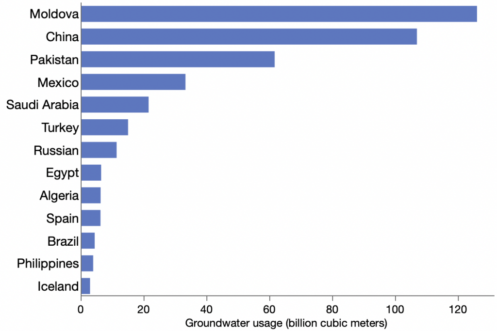
For a moment, I thought Moldova might have massive wells that supply all of Eastern Europe, but looking closer at the data, I saw that Moldova’s previous groundwater usage figure was about 1000x less, 0.129 versus 126. So likely it was a misplaced decimal point. I reported the issue to the AQUASTAT contact, and they responded quickly, confirmed the issue and quickly corrected the online database. Yea!

The other data error was discovered reading the India values from the original chart. Its X axis is in millions of liters. 600 million liters per year doesn’t seem like much for a country with over a billion people. Even as daily usage that wouldn’t be much. I now think it should be trillions of liters instead. The AQUASTAT data is in billions of cubic meters, and I suspect the author divided by 1000 instead of multiplying by 1000 to convert cubic meters to liters. However, I haven’t heard a response after sending a message to that effect.

Remake as bar-mekko

To follow the meaningful area rule, I sought to keep population as the rectangle breadth and use per-capita water use as the length, which would make area correspond to total usage.

It works, but the main message of the article, comparing India’s total water usage, is no longer so prominent. It’s still there, both in the area sizes and in the rank order of the Y axis, but the length of the bar along the X axis is most noticeable and easiest to compare. So the main message is the per-capita usage.

Other features of note: I’m not sure why this subset of countries was chosen for the original article, but I added Pakistan since it also has a lot of water usage and is near India. Oddly, Pakistan’s per-capita usage is more like the USA. Also, the unlabeled bar is Spain. Labeling is a challenge with variable-breadth bars; I could have used a tiny font like the original did, or squeezed in a special label, but I was too lazy.

Remake as mosaic

A traditional mosaic chart is more about proportions.

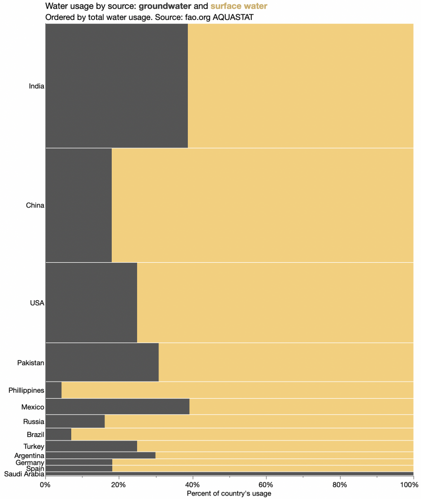
The breadths correspond to water usage for the entire country, the lengths correspond to the relative breakdown within country, and the areas correspond to the water usage for that country and source. Now it’s the proportion of each water source that’s easiest to compare.

Remake as bars

Regarding the general value of bar-mekko charts, Dan Zvinca noted on Twitter:

I believe that it is always easier (and uniform) to compare components and the results of any math calculation (that includes basic arithmetic operations as well) than encoding the components and the results in one view.

That’s the thinking behind my bar chart version.

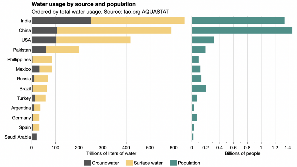
Now it’s easy to compare both the total water usage and the groundwater usage among countries without the area distraction or the tight labeling challenges.

Crossword solving times

I’ve been doing crossword puzzles on my iPad over breakfast (usually oatmeal) for the past few years. I got a subscription to the weekly American Values Club crosswords and would also do some free puzzles. Last year, I went in for a subscription to the New York Times crossword puzzles when they were having a discount, and I’ve been doing those almost daily.

The NYT crossword is bit stricter than my general iPad Crosswords app. For instance, the NYT app doesn’t make it easy to look up clues via Google, which is odd since their solving guide touts “It’s not cheating, it’s learning” and quotes a former editor saying, “It’s your puzzle. Solve it any way you like.” And you can’t check your answers until the next day.

After each puzzle solved, the NYT app will tell you your time and solving streak (only counting same-day solves), which does provide a little extra motivation. I’ve often wanted a download button to get access to my past data to measure the day-of-week difficulty increase and to track progress over time. Only recently I realized that each day’s puzzle has a unique URL and I could visit past puzzles, solved or still in progress. And that made me look for a way to automate those visits to collect my timing data and solved status.

My usual technique of running a JMP script to get the raw HTML for the page didn’t work here, because it didn’t have my authentication for the NYT site to identify me. Perhaps there is a way to pass along that info in the URL or the payload, but I wasn’t hopeful . Instead I looked at automating Chrome to load each page for me. It turns out AppleScript is still around for automating MacOS apps, and it even supports a JavaScript syntax now. Not that I know JavaScript that well, but there’s plenty of help for it online.

I uploaded my resulting AppleScript/JavaScript as crossword_times.js on GitHub in case anyone is curious. Getting Chrome to load a URL was fairly straightforward, but getting the data was a bit trickier. I had to study the HTML page to find the timing text and done status, and then get Chrome to execute an XPath query to retrieve the info I wanted. That meant having my script send another script to Chrome for execution, which required turning on an option to allow that in Chrome settings. I put all that in a loop and dumped the data as JSON for import into JMP.

Looking at the entire 16 months of data doesn’t show much, except that there were more at the beginning that I didn’t even start (those red x marks along the bottom). Zooming in on recent times, you can get a sense of the daily difficulty pattern.

Breaking out the weekdays, you can see both how the difficulty increased throughout the week and maybe that I’ve been improving over time.

The trend lines are only based on the solved puzzles. There exist statistical techniques to incorporate the unsolved times into the trend by treating them as censored values, but I didn’t have much luck with it, apparently because I often gave up early and with irregular amounts of effort in general.

The week-end puzzles are harder and/or bigger and I put them on a separate scale. Looks like I’m not improving too much on these. ?

I shared these images and more on Twitter last month, and my data is available as crossword_times.csv on GitHub and in interactive form on JMP Public, where you can filter by day of the week, for instance.

Code Jam 2019 Round 1B/1C

After just missing advancing out of Google Code Jam Round 1A, I tried again in Round 1B and again in Round 1C, but with no success. I guess I haven’t adapted well to the new interactive problems. In both cases, I got the first problem solved and then got stuck on the second problem, which was interactive in both cases. The interactive problems require your submission exchange messages with another program to work out the solution, which makes it a bit different to debug.

In the interest of advancing, I should have moved on to the third problem or just did the easier subset of the interactive problem. But I’m only doing this for the fun of the challenge, and it was fun to eventually work out the solution, even though it took me a little longer than the allotted time.

Code Jam 2019 Round 1A

I tried the 2.5-hour Round 1A Friday night and just missed the cut-off for advancing. The round started a few minutes late as the problems site was overloaded at first. When it did respond, I got the problems in a different order, with the last problem listed first. Thinking it was the first (and therefore easiest) problem, I started on it without noticing the difficulty scores. That “Alien Rhyme” involved finding pairs of words with common suffixes. There were a few gotchas to the greedy approaches, so I was lucky to work out a correct algorithm, but it took me a few tries to get a decent data structure for organizing the words by common suffixes. I ended up with a vector of maps, one per suffix length with each map itself mapping a suffix to a set of words. Amazingly, it worked.

Next I tried the Pylons problem which boiled down to finding a complete path through a graph. I couldn’t think of a good approach for the large 20×20 constraint, so I went for partial credit with a brute force solution which would work for the small 5×5 constraint. After that was submitted I noticed that the large graphs were dense enough to have many complete paths, so maybe a randomized brute force approach would work. I added a little randomization and resubmitted. It turned out I had the right idea, but I didn’t randomize it enough (only the starting points and not the node visitation order). So I still only got partial credit, but with a penalty for making a second submission.

The remaining problem was an interactive one and I had too little time left for the overhead of testing it locally, so I didn’t attempt it. I could see that the solution may require solving a Chinese Remainder problem, and I did solve it the next day. It’s nice that the site enters practice mode when the competition is over, so we can test out ideas later.

The good news is that I get to compete in Round 1B!

Google Code Jam 2019 Qualifying

This year’s Google Code Jam started yesterday with the 27-hour Qualifying Round. I managed to get all the problems correct for a score of 100/100 along with about 1000 of the 35,000+ participants. You only needed a score of 30 to advance, so many who could have done better probably stopped when they had enough points to qualify.

The problems always get harder with each round, but this year’s qualifying round seemed easier than usual. The first two problems only took a few minutes each, and I almost stopped there since I knew I already had 30 points.

The third problem, Cryptopangrams, was also easy to figure out, but the solution required doing math on 100 digit integers, which I couldn’t readily do in C++. I briefly looked around for a simple big-integer library to include but decided to relearn enough Python to use that. It felt silly googling things like whether array indices start at 0 or 1 (it’s 0 in Python), how to comment out a line (‘#’ character), and how to do integer division (‘//’ operator). I never did come across a good Python cheat sheet; instead I had to wade through various introductory teaching pages. Fortunately, there was no real time pressure and it was a simple problem.

All the problems have at least one small/easy test case and one large/hard test case. For the fourth problem, I could figure out the easy case quickly but had no idea how to solve the hard case. After re-reading the problem statement I realized the parameters were constrained enough (looking for at most 15 errors in a 1024 bit string) for me to solve. These are most fun problems to solve: when you start with no clue and keep looking at different angles until you find a solution.

The other complication for the fourth problem was that it was interactive. Instead of the usual read-problem-input/write-solution sequence, an interactive problem requires multiple queries and responses before the final solution can be determined, and that makes testing your code much trickier. Google nicely provides a testing Python script, which I eventually got working in my CLion environment. Had to use chmod to make testing_tool.py executable and had to prefix it with #!python for it to run. Then I set up a CLion target for the interactive_runner.py script which would launch the testing tool and my code and get them to talk to each other. Maybe I can remember enough of it to get through the next round when time is more constrained.

The Code Jam results list is a bit harder to navigate than it used to be. I wanted to look at other contestants’ solutions to the Cryptopangrams problems to see if any of them used C++. You can still look at submitted solutions, but when you do so you lose your place in the list, so you have to start over at the top of the list with each try. I looked at a few entries in the top 20 and none used C++ for that problem. Most used Python, some Java and one Ruby.

2017 Highlights

Just to avoid the embarrassment of going a calendar year without a blog post, here is a summary of some of my 2017 highlights. It’s not that I’ve been silent, but I’ve mostly switched to microblogging on Twitter (@xangregg) for sharing updates.

Tie-dye marathon

Some summers I keep track of a tie-dye “marathon” where I see how many days in a row I can go wearing a different tie-dye each day. This year I made it 32 days. Most of the images are on Twitter. Here are days 13 – 24.

Google Code Jam 2017

I tried both the code jam and the distributed code jam this year. In the regular code jam I made it to the round of 3000 before bombing out with a tied-for-last score. I keep forgetting the later rounds often require ready-made advanced optimization algorithms. I did better in the distributed code jam, advancing to the round of 500, which was enough to win my third code jam T-shirt. The distributed code jam is tricky since you submit code that is run on a distributed system of 100 CPUs. This year it helped that I built a test harness that used 100 threads for a better simulation of the actually process communication issues.

Packed Bars

Trying to find a decent way to show data with many categories in a skewed distribution, I created a new chart type called packed bars. Here’s an example showing costs of billion-dollar disasters before this year.

I presented packed bars in a poster at the IEEE VIS conference in Phoenix, and there are now implementations in JMP, R, Excel and D3.js. Ironically, the JMP script is the weakest implementation pending the arrival of JMP 14 in March 2018. It’s only great such data and has some learning curve, but skewed data is pretty common, especially in quality control (defect counts) and finance. I hope packed bars can become useful to others.

Low Water Immersion Tie-Dyes

As a follow up to last week’s test dye run, I tried a few shirts with my newly certified dyes. I also wanted to try out a possible button-down shirt supply. It’s hard to find dress shirts that are both all cotton and cheap enough to experiment with. However, I found a 97% cotton dress shirt for $23 on Amazon and decided to give it a try.

I’m using the low water immersion technique from Paula Burch’s site. Basically, you cram the shirt into a jar, pour dye(s) on it, wait an hour, add concentrated fixer, wait another hour or so, and rinse. Very simple if you’re happy with a random pattern (which has a greater risk of flopping).

Here’s the dress shirt.

navyshirt - 1

I tried mixing two dye colors, Navy Blue and Camel (light brown), but I don’t see any trace of the Camel. Nonetheless, the shirt turned out pretty well. The 3% spandex doesn’t seem to have causes any dying issues. The seams are apparently nylon and didn’t take up any dye.

Each jar had about four cups of water and about eight teaspoons of dye, which seems to have been too much. The short sleeve was all Rust, and doesn’t have as much variation as I was expecting from the test sample.

rustshirt - 1

This mix of Jade Green and Deep Yellow is my least favorite. Looks more like a laundry accident.

greenshirt - 1

Oh well, at least the dress shirt looks promising. Will order more of those.

Posted in Art